
Quick Summary & Essential Cheatsheet
Excel contains over 100 statistical formulas, but only ~25 core functions are vital for AP Statistics. Whether analyzing classroom lab data, preparing for digital assessments, or calculating $p$-values and confidence intervals, using the correct sample formulas (like =STDEV.S, =QUARTILE.EXC, =NORM.DIST, and =T.TEST) ensures your calculations mirror the TI-84 Plus graphing calculator and College Board rubrics exactly.
Explore AP Statistics Excel Functions by Unit
- → Master Translation Matrix (TI-84 vs Excel)
- → Live Interactive AP Stats Formula Generator
- → Unit 1: One-Variable Quantitative Data
- → Unit 2: Two-Variable Linear Regression
- → Unit 3 & 4: Probability & Binomial Distribution
- → Unit 5: Normal & Sampling Distributions
- → Unit 6 & 7: Confidence Intervals & t-Tests
- → Unit 8: Chi-Square (χ²) Inference
- → Top 6 Excel Traps to Avoid in AP Stats
- → Frequently Asked Questions
In Advanced Placement (AP) Statistics, students learn that data analysis is about understanding patterns, modeling uncertainty, and drawing reliable statistical inferences. While handheld graphing calculators like the TI-84 Plus CE and TI-Nspire are ubiquitous in test halls, Microsoft Excel remains the industry-standard data analysis tool used in AP capstone research, online college-credit platforms (such as MyStatLab, WebAssign, and ALEKS), and business analytics.
Below is the complete, unit-by-unit guide mapping AP Statistics concepts directly to their exact Excel syntax, complete with parameter definitions, TI-84 equivalents, and real exam problem setups.
AP Statistics to Excel & TI-84 Master Translation Matrix
Use this quick-lookup table to immediately identify which Excel function corresponds to your AP Statistics problem and TI-84 calculator menu command:
| AP Stats Topic | Excel Formula Syntax | TI-84 Equivalent | AP Unit |
|---|---|---|---|
| Sample Mean ($\bar{x}$) | =AVERAGE(A1:A50) |
1-Var Stats → x̄ | Unit 1 |
| Sample Std. Dev. ($s_x$) | =STDEV.S(A1:A50) |
1-Var Stats → Sx | Unit 1 |
| Quartiles ($Q_1, Q_3$) | =QUARTILE.EXC(A1:A50, 1) |
1-Var Stats → Q1, Q3 | Unit 1 |
| Z-Score Standardizing | =STANDARDIZE(x, mean, sd) |
(X - μ) / σ | Unit 1 |
| Correlation ($r$) | =CORREL(array_y, array_x) |
LinReg(a+bx) → r | Unit 2 |
| Coeff. of Determination ($r^2$) | =RSQ(known_y's, known_x's) |
LinReg(a+bx) → r² | Unit 2 |
| Regression Slope ($b_1$) | =SLOPE(known_y's, known_x's) |
LinReg(a+bx) → b | Unit 2 |
| Regression Intercept ($b_0$) | =INTERCEPT(known_y's, known_x's) |
LinReg(a+bx) → a | Unit 2 |
| Combinations ($nCr$) | =COMBIN(n, r) |
MATH → PRB → nCr | Unit 3 |
| Binomial Exact $P(X = k)$ | =BINOM.DIST(k, n, p, FALSE) |
binompdf(n, p, k) | Unit 4 |
| Binomial Cum. $P(X \le k)$ | =BINOM.DIST(k, n, p, TRUE) |
binomcdf(n, p, k) | Unit 4 |
| Normal Cum. $P(X < x)$ | =NORM.DIST(x, μ, σ, TRUE) |
normalcdf(-1E99, x, μ, σ) | Unit 5 |
| Standard Normal $P(Z < z)$ | =NORM.S.DIST(z, TRUE) |
normalcdf(-1E99, z, 0, 1) | Unit 5 |
| Inverse Normal ($z^*$ / cutoff) | =NORM.S.INV(area_to_left) |
invNorm(area, 0, 1) | Unit 5 |
| $t$-Interval Margin of Error | =CONFIDENCE.T(alpha, s, n) |
TInterval → ME | Unit 6 |
| $t$-Dist Critical Value ($t^*$) | =T.INV.2T(alpha, df) |
invT(1 - α/2, df) | Unit 7 |
| 2-Sample $t$-Test $p$-value | =T.TEST(arr1, arr2, 2, 3) |
2-SampTTest (Unequal Var) | Unit 7 |
| Chi-Square Goodness/Indep. $p$-value | =CHISQ.TEST(actuals, expecteds) |
χ²-Test [Observed, Expected] | Unit 8 |
⚡ Interactive AP Stats Excel Formula Generator & Calculator
Select a statistical calculation, adjust your sample inputs, and instantly copy the real-time formula with TI-84 keystrokes!
Unit 1: Exploring One-Variable Quantitative Data
Unit 1 covers measures of center, spread, position, and identifying outliers in univariate distributions.
1. Measures of Center
- Sample Mean ($\bar{x}$):
=AVERAGE(range)— Calculates the arithmetic sum divided by $n$. - Median:
=MEDIAN(range)— Resistant measure of center (50th percentile). - Mode:
=MODE.SNGL(range)— Returns the most frequently occurring value. - Cumulative Frequency / Running Sum:
=SUM($B$2:B2)— Uses an expanding range with an absolute anchor ($B$2) to compute running totals for ogives and cumulative relative frequency plots.
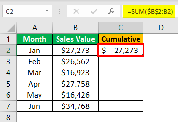
=SUM($B$2:B2)2. Measures of Spread: Why STDEV.S vs STDEV.P Matters!
=STDEV.S and =VAR.S for sample data.
=STDEV.S computes $s = \sqrt{\frac{\sum (x_i - \bar{x})^2}{n - 1}}$ (Bessel's correction). =STDEV.P divides by $N$, assuming you have the entire population. Using STDEV.P on sample data will underestimate variability and lead to incorrect test statistics.
3. Quartiles, IQR, and Outlier Identification
To find the 5-number summary (Min, $Q_1$, Median, $Q_3$, Max):
- First Quartile ($Q_1$):
=QUARTILE.EXC(range, 1) - Third Quartile ($Q_3$):
=QUARTILE.EXC(range, 3) - Interquartile Range (IQR):
=QUARTILE.EXC(range, 3) - QUARTILE.EXC(range, 1) - Lower Outlier Fence:
=Q1 - 1.5 * IQR - Upper Outlier Fence:
=Q3 + 1.5 * IQR
QUARTILE.EXC (exclusive) and QUARTILE.INC (inclusive). For AP Statistics datasets, QUARTILE.EXC closely replicates the median exclusion rule used by TI calculators and AP grading guidelines.
Unit 2: Exploring Two-Variable Data & Linear Regression
In Unit 2, students fit least-squares regression lines ($\hat{y} = a + bx$), assess correlation ($r$), and interpret the coefficient of determination ($r^2$).
| Statistical Parameter | Excel Formula | Parameter Order Note |
|---|---|---|
| Slope ($b_1$) | =SLOPE(known_y's, known_x's) |
Y comes first! Reversing X and Y will invert your slope. |
| Y-Intercept ($b_0$ or $a$) | =INTERCEPT(known_y's, known_x's) |
Y comes first! |
| Correlation ($r$) | =CORREL(array1, array2) |
Order does not matter since $r_{xy} = r_{yx}$. |
| Coeff. of Determination ($r^2$) | =RSQ(known_y's, known_x's) |
Proportion of variation in $y$ explained by linear relationship with $x$. |
| Standard Error of Residuals ($s$) | =STEYX(known_y's, known_x's) |
Estimates typical distance between observed and predicted $y$-values. |
| Predicted Value ($\hat{y}$) | =FORECAST.LINEAR(x_val, known_y's, known_x's) |
Plugs $x$ directly into $\hat{y} = a + bx$. |
Get instant 1-on-1 statistics assignment help →
Unit 3 & 4: Probability, Random Variables & Binomial Distributions
Random simulations and discrete distributions are central to modeling independent binary trials ($B(n, p)$).
1. Random Number Generation for Simulations
=RANDBETWEEN(bottom, top)— Generates a random integer between two bounds (useful for Simple Random Sampling).=COMBIN(n, k)— Calculates the binomial coefficient $\binom{n}{k} = \frac{n!}{k!(n-k)!}$.
2. Binomial Distribution: BINOM.DIST Syntax
Formula syntax: =BINOM.DIST(number_s, trials, probability_s, cumulative)
-
Exact Probability $P(X = k)$: Use
cumulative = FALSE.
Example: Finding the probability of getting exactly 4 heads in 10 flips ($p=0.5$):
=BINOM.DIST(4, 10, 0.5, FALSE)→ 0.2051 (matches TI-84binompdf(10, 0.5, 4)). -
Cumulative Probability $P(X \le k)$: Use
cumulative = TRUE.
Example: Probability of at most 4 heads in 10 flips:
=BINOM.DIST(4, 10, 0.5, TRUE)→ 0.3770 (matches TI-84binomcdf(10, 0.5, 4)). -
"At Least" Probability $P(X \ge k)$: Use complement rule $1 - P(X \le k - 1)$.
Example: Probability of at least 5 heads:
=1 - BINOM.DIST(4, 10, 0.5, TRUE)→ 0.6230. -
Range of Successes $P(a \le X \le b)$:
=BINOM.DIST.RANGE(10, 0.5, 3, 7)
Unit 5: Normal Distribution & Sampling Distributions
For continuous normal models $N(\mu, \sigma)$, Excel separates calculations into the standard normal distribution ($Z \sim N(0, 1)$) and general normal distributions.
| Probability Goal | Excel Formula | TI-84 Equivalent |
|---|---|---|
| $P(X < x)$ (Left-tail area) | =NORM.DIST(x, μ, σ, TRUE) |
normalcdf(-1E99, x, μ, σ) |
| $P(X > x)$ (Right-tail area) | =1 - NORM.DIST(x, μ, σ, TRUE) |
normalcdf(x, 1E99, μ, σ) |
| $P(a < X < b)$ (Between two values) | =NORM.DIST(b, μ, σ, TRUE) - NORM.DIST(a, μ, σ, TRUE) |
normalcdf(a, b, μ, σ) |
| $P(Z < z)$ (Standard Normal) | =NORM.S.DIST(z, TRUE) |
normalcdf(-1E99, z, 0, 1) |
| Find $x$ given percentile $p$ | =NORM.INV(probability, μ, σ) |
invNorm(p, μ, σ) |
| Find critical $z^*$ value | =NORM.S.INV(cumulative_probability) |
invNorm(area, 0, 1) |
- 90% Confidence ($z^*$):
=NORM.S.INV(0.95)→ 1.645 - 95% Confidence ($z^*$):
=NORM.S.INV(0.975)→ 1.960 - 99% Confidence ($z^*$):
=NORM.S.INV(0.995)→ 2.576
Unit 6 & 7: Inference for Means & Proportions (Confidence Intervals & t-Tests)
When standard deviation $\sigma$ is unknown, we estimate spread with sample standard deviation $s$, shifting our inferential model to the Student's $t$-distribution with degrees of freedom $df = n - 1$.
1. Confidence Interval Margin of Error
-
When $\sigma$ is Known ($Z$-Interval):
=CONFIDENCE.NORM(alpha, standard_dev, size)
Example: For 95% confidence ($\alpha = 0.05$), $\sigma = 12$, $n = 36$:=CONFIDENCE.NORM(0.05, 12, 36)→ 3.920. -
When $\sigma$ is Unknown ($t$-Interval - Standard AP Stats):
=CONFIDENCE.T(alpha, s, size)
Example: For 95% confidence ($\alpha = 0.05$), sample $s = 12$, $n = 16$:=CONFIDENCE.T(0.05, 12, 16)→ 6.394.
2. Student's t-Distribution & Critical Values ($t^*$)
- Finding $t^*$ for 2-Tailed Interval:
=T.INV.2T(alpha, df)— For 95% CI with $df = 15$, enter=T.INV.2T(0.05, 15)→ 2.131. - Left-Tail $p$-value:
=T.DIST(t_stat, df, TRUE) - Right-Tail $p$-value:
=T.DIST.RT(t_stat, df) - Two-Tail $p$-value:
=T.DIST.2T(ABS(t_stat), df)
3. Automated Hypothesis Testing with T.TEST
Syntax: =T.TEST(array1, array2, tails, type)
| Type Parameter | Test Performed | When to Use in AP Statistics |
|---|---|---|
type = 1 |
Paired $t$-Test | Pre/post-test scores, matched pairs designs. |
type = 2 |
Two-Sample Pooled Variance ($t$-test) | Assumes equal population variances ($\sigma_1^2 = \sigma_2^2$). Rarely used in AP Stats. |
type = 3 |
Two-Sample Unequal Variance (Welch's $t$-test) | ☆ Standard AP Stats Default! Never pool unless explicitly told to assume equal variance. |
Unit 8: Inference for Categorical Data (Chi-Square χ² Tests)
Chi-square inference assesses Goodness of Fit, Independence, and Homogeneity for categorical counts.
-
Calculate Chi-Square Test $p$-Value from Data:
=CHISQ.TEST(actual_range, expected_range)
Takes your matrix of observed counts and matrix of expected counts $(E = \frac{\text{Row Total} \times \text{Col Total}}{\text{Grand Total}})$ and outputs the exact $p$-value directly! -
Chi-Square Right-Tail Area $P(\chi^2 > x)$:
=CHISQ.DIST.RT(chisq_statistic, df) -
Chi-Square Critical Value:
=CHISQ.INV.RT(alpha, df)
Top 6 Excel Traps That Lose AP Stats Students Points
| Common Excel Mistake ✗ | Correct AP Statistics Approach ✓ |
|---|---|
| Using STDEV.P instead of STDEV.S | Always use =STDEV.S to divide by $n - 1$ for sample data. |
| Entering X before Y in SLOPE and INTERCEPT | Excel formulas require =SLOPE(known_y's, known_x's). Y is always the 1st argument! |
| Confusing NORM.DIST and NORM.S.DIST | Use NORM.DIST(x, μ, σ, TRUE) for raw $x$-values, and NORM.S.DIST(z, TRUE) when already converted to standard $z$-scores. |
| Setting Binomial Cumulative to FALSE for $P(X \le k)$ | Cumulative = TRUE yields $P(X \le k)$, while FALSE yields exact $P(X = k)$. |
| Using Type=2 (Pooled) in T.TEST | Use type = 3 (Welch's unequal variance) to match College Board's 2-Sample $t$-test standard. |
| Forgetting that NORM.DIST yields area to the LEFT | For upper-tail probabilities $P(X > x)$, always compute =1 - NORM.DIST(x, μ, σ, TRUE). |
Frequently Asked Questions
Can you use Microsoft Excel on the AP Statistics Exam?
On the traditional paper-and-pencil AP Statistics exam, students use approved handheld graphing calculators (such as the TI-84 Plus, TI-Nspire, or Casio fx-9750GIII). However, with the transition to College Board digital testing, classroom computer labs, and university-level coursework, Excel proficiency is widely utilized to execute project rubrics, verify homework on Pearson MyMathLab or Canvas, and automate complex inferential calculations.
How do I enable the Data Analysis Toolpak in Excel?
To access automated ANOVA, Descriptive Statistics summaries, and Regression output tables:
- Go to File → Options → Add-ins.
- In the "Manage" drop-down at the bottom, select Excel Add-ins and click Go.
- Check Analysis ToolPak and click OK.
- You will now see the Data Analysis button on the top right of your Data tab!
How do I run a 1-sample t-test in Excel if T.TEST requires two arrays?
Since Excel's =T.TEST expects two arrays, for a 1-sample test against null hypothesis mean $\mu_0$, calculate your $t$-statistic manually with =(AVERAGE(A1:A30) - mu_0) / (STDEV.S(A1:A30) / SQRT(COUNT(A1:A30))), then find the 2-tailed $p$-value with =T.DIST.2T(ABS(t_val), COUNT(A1:A30) - 1).
Related Resources & Tutorials
Need Expert Assistance with AP Statistics or Excel Labs?
Whether you are preparing for your upcoming AP Statistics exam, stuck on complex spreadsheet regression formulas, or need guaranteed A/B grade support on your college online statistics coursework, our vetted statistics tutors are ready 24/7.
Get Statistics Homework & Exam Help Now